In mathematics, particularly linear algebra and numerical analysis, the Gram–Schmidt process is a method fororthonormalising a set of vectors in an inner product space, most commonly the Euclidean space Rn. The Gram–Schmidt process takes a finite, linearly independent set S = {v1, …, vk} for k ≤ n and generates an orthogonal setS′ = {u1, …, uk} that spans the same k-dimensional subspace of Rn as S.
The method is named after Jørgen Pedersen Gram and Erhard Schmidt but it appeared earlier in the work of Laplaceand Cauchy. In the theory of Lie group decompositions it is generalized by the Iwasawa decomposition.[1]
The application of the Gram–Schmidt process to the column vectors of a full column rank matrix yields the QR decomposition (it is decomposed into an orthogonal and a triangular matrix).
In linear algebra, a QR decomposition (also called a QR factorization) of a matrix is a decomposition of a matrix A into a product A = QR of an orthogonal matrix Q and anupper triangular matrix R. QR decomposition is often used to solve the linear least squares problem, and is the basis for a particular eigenvalue algorithm, the QR algorithm.
If A has n linearly independent columns, then the first n columns of Q form an orthonormal basis for the column space of A. More specifically, the first k columns of Q form an orthonormal basis for the span of the first k columns of A for any 1 ≤ k ≤ n.[1] The fact that any column k of A only depends on the first k columns of Q is responsible for the triangular form of R
 .
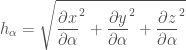
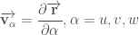
. of any point P(x,y,z) in space as a function of the coordinates u,v,w:
 .
. .
. .
.