Uploaded on Jan 12, 2011
Google Tech Talk
January 6, 2011
Uploaded on Jan 12, 2011
Google Tech Talk
January 6, 2011
The Lamb-Dicke limit is a necessary condition for creation of entangled ions (i.e. the ions must be within the Lamb-Dicke range while their internal and motional states are being manipulated to create the entanglement). The Lamb-Dicke limit defines the upper limit of a range where the ion motion is much smaller than the wavelength of light that is used to excite the desired transition (i.e. the amplitude of the ion motion in the propagation direction of the state manipulating radiation is much less than
λ
/2 Pi, where
λ
is the radiation wavelength). In other words, the Lamb-Dicke limit functionally establishes a maximum temperature for the ions that are to be manipulated. Further, because the ions generally cannot be actively laser cooled while the state manipulations are being performed, the ions must initially be cooled below the Lamb-Dicke limit such that the Lamb-Dicke limit will not be exceeded during the entire manipulation process that creates the entanglement.
π
By Jason Palmer
Science and technology reporter, BBC News, Dallas
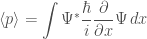
The expected values of position and momentum are given by
In general, any dynamic variable, 

In quantum theory, an experimental setup is described by the observable A to be measured, and the state σ of the system. The expectation value of A in the state σ is denoted as  .
.
Mathematically, A is a self-adjoint operator on a Hilbert space. In the most commonly used case in quantum mechanics, σ is a pure state, described by a normalized[1] vector ψ in the Hilbert space. The expectation value of A in the state ψ is defined as
(1)  .
.
If dynamics is considered, either the vector ψ or the operator A is taken to be time-dependent, depending on whether the Schrödinger picture or Heisenberg picture is used. The time-dependence of the expectation value does not depend on this choice, however.
If A has a complete set of eigenvectors φj, with eigenvalues aj, then (1) can be expressed as
(2)  .
.
This expression is similar to the arithmetic mean, and illustrates the physical meaning of the mathematical formalism: The eigenvalues aj are the possible outcomes of the experiment,[2] and their corresponding coefficient  is the probability that this outcome will occur; it is often called the transition probability.
A particularly simple case arises when A is a projection, and thus has only the eigenvalues 0 and 1. This physically corresponds to a “yes-no” type of experiment. In this case, the expectation value is the probability that the experiment results in “1”, and it can be computed as
(3)  .
.
http://answers.yahoo.com/question/index?qid=20070418194841AAGUVbm
http://en.wikipedia.org/wiki/Expectation_value_(quantum_mechanics)
In quantum mechanics, the particle in a box model (also known as the infinite potential well or the infinite square well) describes a particle free to move in a small space surrounded by impenetrable barriers. The model is mainly used as a hypothetical example to illustrate the differences between classical and quantum systems. In classical systems, for example a ball trapped inside a heavy box, the particle can move at any speed within the box and it is no more likely to be found at one position than another. However, when the well becomes very narrow (on the scale of a few nanometers), quantum effects become important. The particle may only occupy certain positive energy levels. Likewise, it can never have zero energy, meaning that the particle can never “sit still”. Additionally, it is more likely to be found at certain positions than at others, depending on its energy level. The particle may never be detected at certain positions, known as spatial nodes.
The particle in a box model provides one of the very few problems in quantum mechanics which can be solved analytically, without approximations. This means that the observable properties of the particle (such as its energy and position) are related to the mass of the particle and the width of the well by simple mathematical expressions. Due to its simplicity, the model allows insight into quantum effects without the need for complicated mathematics. It is one of the first quantum mechanics problems taught in undergraduate physics courses, and it is commonly used as an approximation for more complicated quantum systems. See also: the history of quantum mechanics.
In quantum mechanics, the wavefunction gives the most fundamental description of the behavior of a particle; the measurable properties of the particle (such as its position, momentum and energy) may all be derived from the wavefunction.[3] The wavefunction ψ(x,t) can be found by solving the Schrödinger equationfor the system

where  is the reduced Planck constant, m is the mass of the particle, i is the imaginary unit and t is time.
Inside the box, no forces act upon the particle, which means that the part of the wavefunction inside the box oscillates through space and time with the same form as a free particle:[1][4]
![\psi(x,t) = [A \sin(kx) + B \cos(kx)]\mathrm{e}^{-\mathrm{i}\omega t},\;](https://i0.wp.com/upload.wikimedia.org/math/8/0/a/80a6430996d2368f8ad3e2b12e3ba842.png)
where A and B are arbitrary complex numbers. The frequency of the oscillations through space and time are given by the wavenumber k and the angular frequency ω respectively. These are both related to the total energy of the particle by the expression

which is known as the dispersion relation for a free particle.[1]

Initial wavefunctions for the first four states in a one-dimensional particle in a box
The size (or amplitude) of the wavefunction at a given position is related to the probability of finding a particle there by P(x,t) = | ψ(x,t) | 2. The wavefunction must therefore vanish everywhere beyond the edges of the box.[1][4] Also, the amplitude of the wavefunction may not “jump” abruptly from one point to the next.[1] These two conditions are only satisfied by wavefunctions with the form

where n is a positive, whole number. The wavenumber is restricted to certain, specific values given by[5]

where L is the size of the box.[7] Negative values of n are neglected, since they give wavefunctions identical to the positive n solutions except for a physically unimportant sign change.[6]
Finally, the unknown constant A may be found by normalizing the wavefunction so that the total probability density of finding the particle in the system is 1. It follows that

Thus, A may be any complex number with absolute value √(2/L); these different values of A yield the same physical state, so A = √(2/L) can be selected to simplify.

The energy of a particle in a box (black circles) and a free particle (grey line) both depend upon wavenumber in the same way. However, the particle in a box may only have certain, discrete energy levels.
The energies which correspond with each of the permitted wavenumbers may be written as[5]
 .
.The energy levels increase with n2, meaning that high energy levels are separated from each other by a greater amount than low energy levels are. The lowest possible energy for the particle (its zero-point energy) is found in state 1, which is given by[8]

The particle, therefore, always has a positive energy. This contrasts with classical systems, where the particle can have zero energy by resting motionless at the bottom of the box. This can be explained in terms of the uncertainty principle, which states that the product of the uncertainties in the position and momentum of a particle is limited by

It can be shown that the uncertainty in the position of the particle is proportional to the width of the box.[9] Thus, the uncertainty in momentum is roughly inversely proportional to the width of the box.[8] The kinetic energy of a particle is given by E = p2 / (2m), and hence the minimum kinetic energy of the particle in a box is inversely proportional to the mass and the square of the well width, in qualitative agreement with the calculation above.[8]
In classical physics, the particle can be detected anywhere in the box with equal probability. In quantum mechanics, however, the probability density for finding a particle at a given position is derived from the wavefunction as P(x) = | ψ(x) | 2. For the particle in a box, the probability density for finding the particle at a given position depends upon its state, and is given by

Thus, for any value of n greater than one, there are regions within the box for which P(x) = 0, indicating that spatial nodes exist at which the particle cannot be found.
In quantum mechanics, the average, or expectation value of the position of a particle is given by

For the particle in a box, it can be shown that the average position is always  , regardless of the state of the particle. In other words, the average position at which a particle in a box may be detected is exactly in the center of the quantum well; in agreement with a classical system.
If a particle is trapped in a two-dimensional box, it may freely move in the x and y-directions, between barriers separated by lengths Lx andLy respectively. Using a similar approach to that of the one-dimensional box, it can be shown that the wavefunctions and energies are given respectively by
 ,
, ,
,where the two-dimensional wavevector is given by
 .
.For a three dimensional box, the solutions are
 ,
, ,
,where the three-dimensional wavevector is given by
 .
.An interesting feature of the above solutions is that when two or more of the lengths are the same (e.g. Lx = Ly), there are multiple wavefunctions corresponding to the same total energy. For example the wavefunction with nx = 2,ny = 1 has the same energy as the wavefunction with nx = 1,ny = 2. This situation is called degeneracy and for the case where exactly two degenerate wavefunctions have the same energy that energy level is said to be doubly degenerate. Degeneracy results from symmetry in the system. For the above case two of the lengths are equal so the system is symmetric with respect to a 90° rotation.
http://en.wikipedia.org/wiki/Particle_in_a_box
http://en.wikipedia.org/wiki/Quantum_harmonic_oscillator
Modern Quantum Mechanics (2nd Edition)
Quantum Mechanics Non-Relativistic Theory, Third Edition: Volume 3
The Stark effect is the shifting and splitting of spectral lines of atoms and molecules due to the presence of an external static electric field. The amount of splitting and or shifting is called the Stark splitting or Stark shift. In general one distinguishes first- and second-order Stark effects. The first-order effect is linear in the applied electric field, while the second-order effect is quadratic in the field.
The Stark effect is responsible for the pressure broadening (Stark broadening) of spectral lines by charged particles. When the split/shifted lines appear in absorption, the effect is called the inverse Stark effect.
The Stark effect is the electric analogue of the Zeeman effect where a spectral line is split into several components due to the presence of a magnetic field.
The Stark effect can be explained with fully quantum mechanical approaches, but it has also been a fertile testing ground for semiclassical methods.
The Stark effect originates from the interaction between a charge distribution (atom or molecule) and an external electric field. Before turning to quantum mechanics we describe the interaction classically and consider a continuous charge distribution ρ(r). If this charge distribution is non-polarizable its interaction energy with an external electrostatic potential V(r) is

If the electric field is of macroscopic origin and the charge distribution is microscopic, it is reasonable to assume that the electric field is uniform over the charge distribution. That is, V is given by a two-term Taylor expansion,

where we took the origin 0 somewhere within ρ. Setting  as the zero energy, the interaction becomes

Here we have introduced the dipole moment μ of ρ as an integral over the charge distribution. In case ρ consists of N point charges qj this definition becomes a sum

Turning now to quantum mechanics we see an atom or a molecule as a collection of point charges (electrons and nuclei), so that the second definition of the dipole applies. The interaction of atom or molecule with a uniform external field is described by the operator

This operator is used as a perturbation in first- and second-order perturbation theory to account for the first- and second-order Stark effect.
Let the unperturbed atom or molecule be in a g-fold degenerate state with orthonormal zeroth-order state functions  . (Non-degeneracy is the special case g = 1). According to perturbation theory the first-order energies are the eigenvalues of the g x g matrix with general element

If g = 1 (as is often the case for electronic states of molecules) the first-order energy becomes proportional to the expectation (average) value of the dipole operator  ,
,

Because a dipole moment is a polar vector, the diagonal elements of the perturbation matrix Vint vanish for systems with an inversion center (such as atoms). Molecules with an inversion center in a non-degenerate electronic state do not have a (permanent) dipole and hence do not show a linear Stark effect.
In order to obtain a non-zero matrix Vint for systems with an inversion center it is necessary that some of the unperturbed functions  have opposite parity (obtain plus and minus under inversion), because only functions of opposite parity give non-vanishing matrix elements. Degenerate zeroth-order states of opposite parity occur for excited hydrogen-like (one-electron) atoms. Such atoms have the principal quantum number n among their quantum numbers. The excited state of hydrogen-like atoms with principal quantum number n is n2-fold degenerate and

where  is the azimuthal (angular momentum) quantum number. For instance, the excited n = 4 state contains the following states,

The one-electron states with even are even under parity, while those with odd are odd under parity. Hence hydrogen-like atoms with n>1 show first-order Stark effect.
The first-order Stark effect occurs in rotational transitions of symmetric top molecules (but not for linear and asymmetric molecules). In first approximation a molecule may be seen as a rigid rotor. A symmetric top rigid rotor has the unperturbed eigenstates

with 2(2J+1)-fold degenerate energy for |K| > 0 and (2J+1)-fold degenerate energy for K=0. Here DJMK is an element of the Wigner D-matrix. The first-order perturbation matrix on basis of the unperturbed rigid rotor function is non-zero and can be diagonalized. This gives shifts and splittings in the rotational spectrum. Quantitative analysis of these Stark shift yields the permanent electric dipole moment of the symmetric top molecule.
As stated, the quadratic Stark effect is described by second-order perturbation theory. The zeroth-order problems

are assumed to be solved. It is usual to assume that the zeroth-order state to be perturbed is non-degenerate. If we take the ground state as the non-degenerate state under consideration (for hydrogen-like atoms: n = 1), perturbation theory gives

with the components of the polarizability tensor α defined by

The energy E(2) gives the quadratic Stark effect.
Because of their spherical symmetry the polarizability tensor of atoms is isotropic,

which is the quadratic Stark shift for atoms. For many molecules this expression is not too bad an approximation, because molecular tensors are often reasonably isotropic.
The perturbative treatment of the Stark effect has some problems. In the presence of an electric field, states of atoms and molecules that were previously bound (square-integrable), become formally (non-square-integrable) resonances of finite width. These resonances may decay in finite time via field ionization. For low lying states and not too strong fields the decay times are so long, however, that for all practical purposes the system can be regarded as bound. For highly excited states and/or very strong fields ionization may have to be accounted for. (See also the article on the Rydberg atom).
Modern Quantum Mechanics (2nd Edition)
the canonical commutation relation is the relation between canonical conjugate quantities (quantities which are related by definition such that one is the Fourier transform of another), for example:
![[x,p_x] = i\hbar](https://i0.wp.com/upload.wikimedia.org/math/a/5/4/a54264a655e2e824a033aa70f53e51d5.png)
between the position x and momentum px in the x direction of a point particle in one dimension, where [x,px] = xpx − pxx is the commutator of x and px, i is the imaginary unit, and ħ is the reducedPlanck’s constant h /2π . This relation is attributed to Max Born, and it was noted by E. Kennard (1927) to imply the Heisenberg uncertainty principle.
By contrast, in classical physics, all observables commute and the commutator would be zero. However, an analogous relation exists, which is obtained by replacing the commutator with the Poisson bracket multiplied by i ħ:

This observation led Dirac to propose that the quantum counterparts  of classical observables f, g satisfy
![[\hat f,\hat g]= i\hbar\widehat{\{f,g\}} \, .](https://i0.wp.com/upload.wikimedia.org/math/d/6/7/d67e60da2040fa460436544adb0a6fb4.png)
According to the standard mathematical formulation of quantum mechanics, quantum observables such as x and p should be represented as self-adjoint operators on some Hilbert space. It is relatively easy to see that two operators satisfying the canonical commutation relations cannot both be bounded. The canonical commutation relations can be made tamer by writing them in terms of the (bounded) unitary operators e − ikx and e − iap. The result is the so-called Weyl relations. The uniqueness of the canonical commutation relations between position and momentum is guaranteed by theStone-von Neumann theorem. The group associated with the commutation relations is called the Heisenberg group.
![[{L_x}, {L_y}] = i \hbar \epsilon_{xyz} {L_z},](https://i0.wp.com/upload.wikimedia.org/math/c/9/e/c9e1b0ea439209810a0c85585d306ee7.png)
where εxyz is the Levi-Civita symbol and simply reverses the sign of the answer under pairwise interchange of the indices. An analogous relation holds for the spin operators.
All such nontrivial commutation relations for pairs of operators lead to corresponding uncertainty relations (H. P. Robertson[2]), involving positive semi-definite expectation contributions by their respective commutators and anticommutators. In general, for two Hermitian operators A and B, consider expectation values in a system in the state ψ, the variances around the corresponding expectation values being (ΔA)2 ≡ 〈 (A −<A>)2 〉, etc.
Then
![\Delta A \, \Delta B \geq \frac{1}{2} \sqrt{ \left|\left\langle\left[{A},{B}\right]\right\rangle \right|^2 + \left|\left\langle\left\{ A-\langle A\rangle ,B-\langle B\rangle \right\} \right\rangle \right|^2} ,](https://i0.wp.com/upload.wikimedia.org/math/3/c/e/3ce32bd650db6f4914a8964900c639f5.png)
where [A,B] ≡ AB−BA is the commutator of A and B, and {A,B} ≡ AB+BA is the anticommutator. This follows through use of the Cauchy–Schwarz inequality, since |〈A2〉| |〈B2〉| ≥ |〈AB〉|2, and AB = ([A,B] + {A,B}) /2 ; and similarly for the shifted operators A−〈A〉 and B−〈B〉 . Judicious choices for A and B yield Heisenberg’s familiar uncertainty relation, for x and p, as usual; or, here, Lx and Ly , in angular momentum multiplets, ψ = |l , m 〉 , useful constraints such as l (l+1) ≥ m (m+1), and hence l ≥ m, among others.
Modern Quantum Mechanics (2nd Edition)
http://www.dfcd.net/articles/firstyear/lectures/angmom.pdf
http://en.wikipedia.org/wiki/Canonical_commutation_relation
http://galileo.phys.virginia.edu/classes/751.mf1i.fall02/AngularMomentum.htm
Because an arbitrary potential can be approximated as a harmonic potential at the vicinity of a stable equilibrium point, it is one of the most important model systems in quantum mechanics.
In the one-dimensional harmonic oscillator problem, a particle of mass m is subject to a potential V(x) given by

where ω is the angular frequency of the oscillator. In classical mechanics,  is called the spring stiffness coefficient, force constant or spring constant, and
  the angular frequency.
The Hamiltonian of the particle is:

where  is the position operator, and
  is the momentum operator, given by

The first term in the Hamiltonian represents the kinetic energy of the particle, and the second term represents the potential energy in which it resides. In order to find the energy levels and the corresponding energy eigenstates, we must solve the time-independent Schrödinger equation,

We can solve the differential equation in the coordinate basis, using a spectral method. It turns out that there is a family of solutions. In the position basis they are

The functions Hn are the physicists’ Hermite polynomials:

The corresponding energy levels are
 .
.http://en.wikipedia.org/wiki/Quantum_harmonic_oscillator
Modern Quantum Mechanics (2nd Edition)
Quantum Mechanics Non-Relativistic Theory, Third Edition: Volume 3
Introduction to Quantum Mechanics (2nd Edition)
Introductory Quantum Mechanics (4th Edition)
Perspectives of Modern Physics, Sec 8-7
In the standardinterpretation of quantum mechanics, the quantum state, also called awavefunction or state vector, is the most complete description that can be given to a physical system.
The most general form is the time-dependent Schrödinger equation, which gives a description of a system evolving with time. For systems in astationary state, the time-independent Schrödinger equation is sufficient. Approximate solutions to the time-independent Schrödinger equation are commonly used to calculate the energy levels and other properties of atoms and molecules.
Schrödinger’s equation can be mathematically transformed into Werner Heisenberg‘s matrix mechanics, and into Richard Feynman‘s path integral formulation. The Schrödinger equation describes time in a way that is inconvenient for relativistic theories, a problem which is not as severe in matrix mechanics and completely absent in the path integral formulation.
http://en.wikipedia.org/wiki/Schr%C3%B6dinger_equation
Modern Quantum Mechanics (2nd Edition)
Quantum Mechanics Non-Relativistic Theory, Third Edition: Volume 3
http://en.wikipedia.org/wiki/Hydrogen_atom
Modern Quantum Mechanics (2nd Edition)
Quantum Mechanics Non-Relativistic Theory, Third Edition: Volume 3